Evaluating model performance - predicting Boston housing prices
In this project, you evaluate the performance and predictive power of a model that has been trained and tested on data collected from homes in suburbs of Boston, Massachusetts. A model trained on this data that is seen as a good fit could then be used to make certain predictions about a home — in particular, its monetary value. This model would prove to be invaluable for someone like a real estate agent who could make use of such information on a daily basis. Here is the code for this project which was a part of Udacity’s Machine Learning Engineer Nanodegree.
The dataset for this project originates from the UCI Machine Learning Repository. The Boston housing data was collected in 1978 and each of the 506 entries represent aggregated data about 14 features for homes from various suburbs in Boston, Massachusetts. For the purposes of this project, the following preprocessing steps have been made to the dataset:
- 16 data points have an
'MEDV'value of 50.0. These data points likely contain missing or censored values and have been removed. - 1 data point has an
'RM'value of 8.78. This data point can be considered an outlier and has been removed. - The features
'RM','LSTAT','PTRATIO', and'MEDV'are essential. The remaining non-relevant features have been excluded. - The feature
'MEDV'has been multiplicatively scaled to account for 35 years of market inflation.
Run the code cell below to load the Boston housing dataset, along with a few of the necessary Python libraries required for this project. You will know the dataset loaded successfully if the size of the dataset is reported.
# Import libraries necessary for this projectimport numpy as npimport pandas as pdfrom sklearn.cross_validation import ShuffleSplit
# Import supplementary visualizations code visuals.pyimport visuals as vs
# Pretty display for notebooks%matplotlib inline
# Load the Boston housing datasetdata = pd.read_csv('housing.csv')prices = data['MEDV']features = data.drop('MEDV', axis = 1)
# Successprint "Boston housing dataset has {} data points with {} variables each.".format(*data.shape)
Boston housing dataset has 489 data points with 4 variables each.Data Exploration
In this first section of this project, you will make a cursory investigation about the Boston housing data and provide your observations. Familiarizing yourself with the data through an explorative process is a fundamental practice to help you better understand and justify your results.
Since the main goal of this project is to construct a working model which has the capability of predicting the value of houses, we will need to separate the dataset into features and the target variable. The features, 'RM', 'LSTAT', and 'PTRATIO', give us quantitative information about each data point. The target variable, 'MEDV', will be the variable we seek to predict. These are stored in features and prices, respectively.
Implementation: Calculate Statistics
For your very first coding implementation, you will calculate descriptive statistics about the Boston housing prices. Since numpy has already been imported for you, use this library to perform the necessary calculations. These statistics will be extremely important later on to analyze various prediction results from the constructed model.
In the code cell below, you will need to implement the following:
- Calculate the minimum, maximum, mean, median, and standard deviation of
'MEDV', which is stored inprices.- Store each calculation in their respective variable.
# TODO: Minimum price of the dataminimum_price = np.min(prices)
# TODO: Maximum price of the datamaximum_price = np.max(prices)
# TODO: Mean price of the datamean_price = np.mean(prices)
# TODO: Median price of the datamedian_price = np.median(prices)
# TODO: Standard deviation of prices of the datastd_price = np.std(prices)
# Show the calculated statisticsprint "Statistics for Boston housing dataset:\n"print "Minimum price: ${:,.2f}".format(minimum_price)print "Maximum price: ${:,.2f}".format(maximum_price)print "Mean price: ${:,.2f}".format(mean_price)print "Median price ${:,.2f}".format(median_price)print "Standard deviation of prices: ${:,.2f}".format(std_price)
Statistics for Boston housing dataset:
Minimum price: $105,000.00Maximum price: $1,024,800.00Mean price: $454,342.94Median price $438,900.00Standard deviation of prices: $165,171.13Question 1 - Feature Observation
As a reminder, we are using three features from the Boston housing dataset: 'RM', 'LSTAT', and 'PTRATIO'. For each data point (neighborhood):
'RM'is the average number of rooms among homes in the neighborhood.'LSTAT'is the percentage of homeowners in the neighborhood considered “lower class” (working poor).'PTRATIO'is the ratio of students to teachers in primary and secondary schools in the neighborhood.
Using your intuition, for each of the three features above, do you think that an increase in the value of that feature would lead to an increase in the value of 'MEDV' or a decrease in the value of 'MEDV'? Justify your answer for each.
Hint: Would you expect a home that has an 'RM' value of 6 be worth more or less than a home that has an 'RM' value of 7?
**Answer: **
- ‘RM’: Increase. More rooms == Higher value homes
- ’LSTAT’: Decrease. Less income == Less buying power == Lesser value homes
- ’PTRATIO’: Decrease. More students == lower quality/cheaper schools == cheaper neighborhood
Developing a Model
In this second section of the project, you will develop the tools and techniques necessary for a model to make a prediction. Being able to make accurate evaluations of each model’s performance through the use of these tools and techniques helps to greatly reinforce the confidence in your predictions.
Implementation: Define a Performance Metric
It is difficult to measure the quality of a given model without quantifying its performance over training and testing. This is typically done using some type of performance metric, whether it is through calculating some type of error, the goodness of fit, or some other useful measurement. For this project, you will be calculating the coefficient of determination, R2, to quantify your model’s performance. The coefficient of determination for a model is a useful statistic in regression analysis, as it often describes how “good” that model is at making predictions.
The values for R2 range from 0 to 1, which captures the percentage of squared correlation between the predicted and actual values of the target variable. A model with an R2 of 0 is no better than a model that always predicts the mean of the target variable, whereas a model with an R2 of 1 perfectly predicts the target variable. Any value between 0 and 1 indicates what percentage of the target variable, using this model, can be explained by the features. A model can be given a negative R2 as well, which indicates that the model is arbitrarily worse than one that always predicts the mean of the target variable.
For the performance_metric function in the code cell below, you will need to implement the following:
- Use
r2_scorefromsklearn.metricsto perform a performance calculation betweeny_trueandy_predict. - Assign the performance score to the
scorevariable.
# TODO: Import 'r2_score'from sklearn.metrics import r2_score
def performance_metric(y_true, y_predict):    """ Calculates and returns the performance score between        true and predicted values based on the metric chosen. """
    # TODO: Calculate the performance score between 'y_true' and 'y_predict'    score = r2_score(y_true, y_predict)
    # Return the score    return score
Question 2 - Goodness of Fit
Assume that a dataset contains five data points and a model made the following predictions for the target variable:
| True Value | Prediction |
|---|---|
| 3.0 | 2.5 |
| -0.5 | 0.0 |
| 2.0 | 2.1 |
| 7.0 | 7.8 |
| 4.2 | 5.3 |
Would you consider this model to have successfully captured the variation of the target variable? Why or why not?
Run the code cell below to use the performance_metric function and calculate this model’s coefficient of determination.
# Calculate the performance of this modelscore = performance_metric([3, -0.5, 2, 7, 4.2], [2.5, 0.0, 2.1, 7.8, 5.3])print "Model has a coefficient of determination, R^2, of {:.3f}.".format(score)Model has a coefficient of determination, R^2, of 0.923.Answer: Yes, as r2_value is very close to 1. This r2_value means that the model explains 92.3% of the target variable.
Implementation: Shuffle and Split Data
Your next implementation requires that you take the Boston housing dataset and split the data into training and testing subsets. Typically, the data is also shuffled into a random order when creating the training and testing subsets to remove any bias in the ordering of the dataset.
For the code cell below, you will need to implement the following:
- Use
train_test_splitfromsklearn.cross_validationto shuffle and split thefeaturesandpricesdata into training and testing sets.- Split the data into 80% training and 20% testing.
- Set the
random_statefortrain_test_splitto a value of your choice. This ensures results are consistent.
- Assign the train and testing splits to
X_train,X_test,y_train, andy_test.
# TODO: Import 'train_test_split'from sklearn.cross_validation import train_test_split
# TODO: Shuffle and split the data into training and testing subsetsX_train, X_test, y_train, y_test = train_test_split(features, prices, test_size=0.2, random_state=0)
# Successprint "Training and testing split was successful."
Training and testing split was successful.Question 3 - Training and Testing
What is the benefit to splitting a dataset into some ratio of training and testing subsets for a learning algorithm?
Hint: What could go wrong with not having a way to test your model?
**Answer: **
- We can evaluate the model by using it to predict values for the testing subset which is unseen data.
- Without testing we wouldn’t know how the model would perform on unseen data.
- Testing on just the training data would likely result in (misleading) high accuracy scores because of overfitting.
Analyzing Model Performance
In this third section of the project, you’ll take a look at several models’ learning and testing performances on various subsets of training data. Additionally, you’ll investigate one particular algorithm with an increasing 'max_depth' parameter on the full training set to observe how model complexity affects performance. Graphing your model’s performance based on varying criteria can be beneficial in the analysis process, such as visualizing behavior that may not have been apparent from the results alone.
Learning Curves
The following code cell produces four graphs for a decision tree model with different maximum depths. Each graph visualizes the learning curves of the model for both training and testing as the size of the training set is increased. Note that the shaded region of a learning curve denotes the uncertainty of that curve (measured as the standard deviation). The model is scored on both the training and testing sets using R2, the coefficient of determination.
Run the code cell below and use these graphs to answer the following question.
# Produce learning curves for varying training set sizes and maximum depthsvs.ModelLearning(features, prices)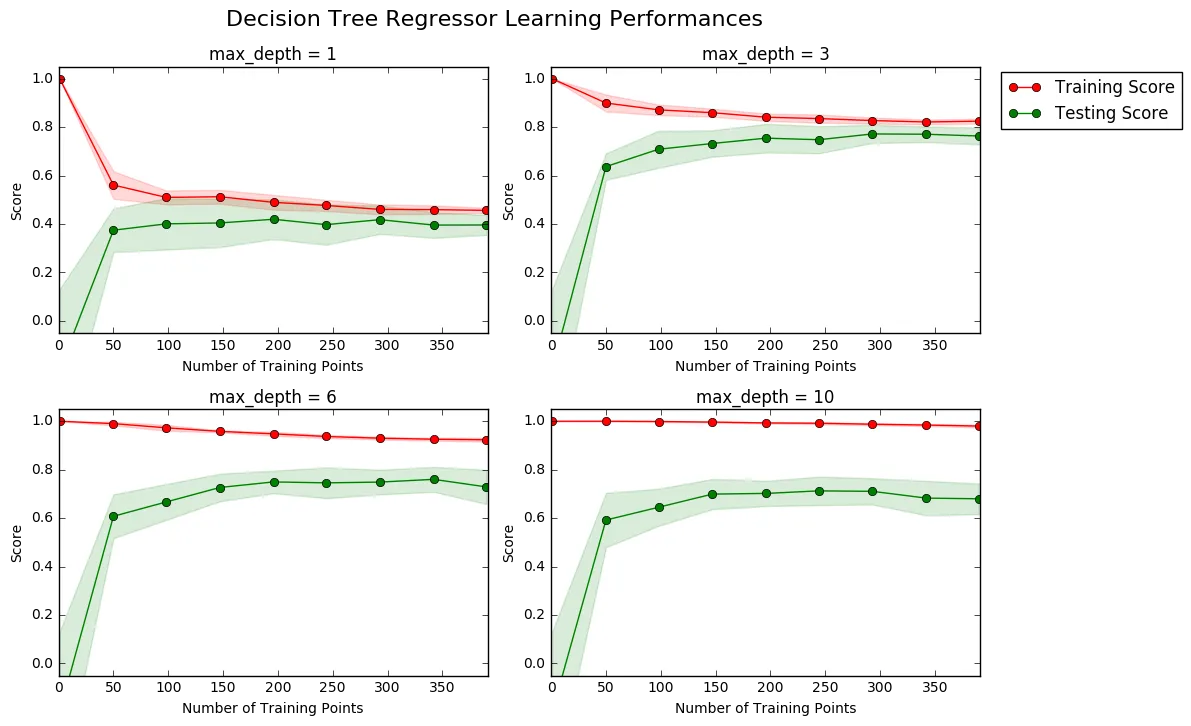
Question 4 - Learning the Data
Choose one of the graphs above and state the maximum depth for the model. What happens to the score of the training curve as more training points are added? What about the testing curve? Would having more training points benefit the model?
Hint: Are the learning curves converging to particular scores?
**Answer: ** max_depth = 3 Training curve decreases slightly until it becomes steady at 0.8. Testing curve increases rapidly at first until it converges with the training curve at 0.8. More training points wouldn’t benefit the model as the score is already closer to 1 and both curves have converged.
Complexity Curves
The following code cell produces a graph for a decision tree model that has been trained and validated on the training data using different maximum depths. The graph produces two complexity curves — one for training and one for validation. Similar to the learning curves, the shaded regions of both the complexity curves denote the uncertainty in those curves, and the model is scored on both the training and validation sets using the performance_metric function.
Run the code cell below and use this graph to answer the following two questions.
vs.ModelComplexity(X_train, y_train)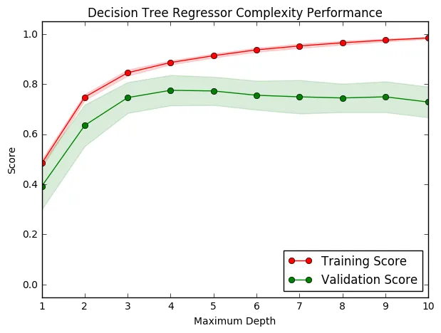
Question 5 - Bias-Variance Tradeoff
When the model is trained with a maximum depth of 1, does the model suffer from high bias or from high variance? How about when the model is trained with a maximum depth of 10? What visual cues in the graph justify your conclusions?
Hint: How do you know when a model is suffering from high bias or high variance?
**Answer: **
max_depth = 1
Both scores are < 0.5 == not complex enough (Underfitting) == High bias
max_depth = 10
Training score is almost 1 but validation score is much lower == too complex (Overfitting) == High variance
Question 6 - Best-Guess Optimal Model
Which maximum depth do you think results in a model that best generalizes to unseen data? What intuition lead you to this answer?
**Answer: **
max_depth = 4
Model complexity: At this value, the testing score is the maximum == model performs best against unseen data.
Evaluating Model Performance
In this final section of the project, you will construct a model and make a prediction on the client’s feature set using an optimized model from fit_model.
Question 7 - Grid Search
What is the grid search technique and how it can be applied to optimize a learning algorithm?
**Answer: ** Grid search technique is applying multiple sets of parameters to an algorithm, cross validating each set to find out which set of parameters gives the best performance.
This can be used to optimize a learning algorithm by choosing a set of parameters for the algorithm and finding the set that gives the best perfomance and using those parameters for prediction.
# list of parameters to search from, below example is 2x2=4 sets of parametersparameters = {'kernel':('linear', 'rbf'), 'C':[1, 10]}# algorithm to usesvr = svm.SVC()# classifier with algorithm and parametersclf = grid_search.GridSearchCV(svr, parameters)# tries all parameter combinationsclf.fit(iris.data, iris.target)# access best parametersprint clf.best_params_In the above example, all four sets of parameters are used, and the set of parameters with the highest score (r2_score/accuracy_score) is the best set of parameters.
Question 8 - Cross-Validation
What is the k-fold cross-validation training technique? What benefit does this technique provide for grid search when optimizing a model?
Hint: Much like the reasoning behind having a testing set, what could go wrong with using grid search without a cross-validated set?
**Answer: **
Instead of just splitting into 20% testing, 80% training, k-fold uses all data as training and testing data by running k separate learning experiments and calculating the average.
Ex. 200 data points, k=10 give 10 bins of 20 data points each.
Each time only one of the k bins is used for testing and the rest for training. This way each ‘bin’ is used exactly once for testing.
Benefits: Prevents overfitting on the training set used and the model is more generalized.
Implementation: Fitting a Model
Your final implementation requires that you bring everything together and train a model using the decision tree algorithm. To ensure that you are producing an optimized model, you will train the model using the grid search technique to optimize the 'max_depth' parameter for the decision tree. The 'max_depth' parameter can be thought of as how many questions the decision tree algorithm is allowed to ask about the data before making a prediction. Decision trees are part of a class of algorithms called supervised learning algorithms.
In addition, you will find your implementation is using ShuffleSplit() for an alternative form of cross-validation (see the 'cv_sets' variable). While it is not the K-Fold cross-validation technique you describe in Question 8, this type of cross-validation technique is just as useful!. The ShuffleSplit() implementation below will create 10 ('n_splits') shuffled sets, and for each shuffle, 20% ('test_size') of the data will be used as the validation set. While you’re working on your implementation, think about the contrasts and similarities it has to the K-fold cross-validation technique.
Please note that ShuffleSplit has different parameters in scikit-learn versions 0.17 and 0.18.
For the fit_model function in the code cell below, you will need to implement the following:
- Use
DecisionTreeRegressorfromsklearn.treeto create a decision tree regressor object.- Assign this object to the
'regressor'variable.
- Assign this object to the
- Create a dictionary for
'max_depth'with the values from 1 to 10, and assign this to the'params'variable. - Use
make_scorerfromsklearn.metricsto create a scoring function object.- Pass the
performance_metricfunction as a parameter to the object. - Assign this scoring function to the
'scoring_fnc'variable.
- Pass the
- Use
GridSearchCVfromsklearn.grid_searchto create a grid search object.- Pass the variables
'regressor','params','scoring_fnc', and'cv_sets'as parameters to the object. - Assign the
GridSearchCVobject to the'grid'variable.
- Pass the variables
# TODO: Import 'make_scorer', 'DecisionTreeRegressor', and 'GridSearchCV'from sklearn.tree import DecisionTreeRegressorfrom sklearn.metrics import make_scorerfrom sklearn.grid_search import GridSearchCV
def fit_model(X, y):    """ Performs grid search over the 'max_depth' parameter for a        decision tree regressor trained on the input data [X, y]. """
    # Create cross-validation sets from the training data    cv_sets = ShuffleSplit(X.shape[0], n_iter = 10, test_size = 0.20, random_state = 30)
    # TODO: Create a decision tree regressor object    regressor = DecisionTreeRegressor()
    # TODO: Create a dictionary for the parameter 'max_depth' with a range from 1 to 10    params = {'max_depth': range(1, 11)}
    # TODO: Transform 'performance_metric' into a scoring function using 'make_scorer'    scoring_fnc = make_scorer(performance_metric)
    # TODO: Create the grid search object    grid = GridSearchCV(regressor, params, scoring=scoring_fnc, cv=cv_sets)
    # Fit the grid search object to the data to compute the optimal model    grid = grid.fit(X, y)
    # Return the optimal model after fitting the data    return grid.best_estimator_
Making Predictions
Once a model has been trained on a given set of data, it can now be used to make predictions on new sets of input data. In the case of a decision tree regressor, the model has learned what the best questions to ask about the input data are, and can respond with a prediction for the target variable. You can use these predictions to gain information about data where the value of the target variable is unknown — such as data the model was not trained on.
Question 9 - Optimal Model
What maximum depth does the optimal model have? How does this result compare to your guess in Question 6?
Run the code block below to fit the decision tree regressor to the training data and produce an optimal model.
# Fit the training data to the model using grid searchreg = fit_model(X_train, y_train)
# Produce the value for 'max_depth'print "Parameter 'max_depth' is {} for the optimal model.".format(reg.get_params()['max_depth'])
Parameter 'max_depth' is 4 for the optimal model.**Answer: ** Same as my guess
Question 10 - Predicting Selling Prices
Imagine that you were a real estate agent in the Boston area looking to use this model to help price homes owned by your clients that they wish to sell. You have collected the following information from three of your clients:
| Feature | Client 1 | Client 2 | Client 3 |
|---|---|---|---|
| Total number of rooms in home | 5 rooms | 4 rooms | 8 rooms |
| Neighborhood poverty level (as %) | 17% | 32% | 3% |
| Student-teacher ratio of nearby schools | 15-to-1 | 22-to-1 | 12-to-1 |
What price would you recommend each client sell his/her home at? Do these prices seem reasonable given the values for the respective features?
Hint: Use the statistics you calculated in the Data Exploration section to help justify your response.
Run the code block below to have your optimized model make predictions for each client’s home.
# Produce a matrix for client dataclient_data = [[5, 17, 15], # Client 1               [4, 32, 22], # Client 2               [8, 3, 12]]  # Client 3
# Show predictionsfor i, price in enumerate(reg.predict(client_data)):    print "Predicted selling price for Client {}'s home: ${:,.2f}".format(i+1, price)
Predicted selling price for Client 1's home: $391,183.33Predicted selling price for Client 2's home: $189,123.53Predicted selling price for Client 3's home: $942,666.67Answer:
Recommendations:
- Client 1: $391,183.33
- Client 2: $189,123.53
- Client 3: $942,666.67
Very reasonable based on my answers for Question 1.
Client 2: Less rooms, high poverty level, high student
Client 3: Many rooms, very low poverty level, less student == close to the max value
Client 1: Rooms/poverty level/student values in between values for clients 2&3 == home value falls in between
Sensitivity
An optimal model is not necessarily a robust model. Sometimes, a model is either too complex or too simple to sufficiently generalize to new data. Sometimes, a model could use a learning algorithm that is not appropriate for the structure of the data given. Other times, the data itself could be too noisy or contain too few samples to allow a model to adequately capture the target variable — i.e., the model is underfitted. Run the code cell below to run the fit_model function ten times with different training and testing sets to see how the prediction for a specific client changes with the data it’s trained on.
vs.PredictTrials(features, prices, fit_model, client_data)Trial 1: $391,183.33Trial 2: $419,700.00Trial 3: $415,800.00Trial 4: $420,622.22Trial 5: $418,377.27Trial 6: $411,931.58Trial 7: $399,663.16Trial 8: $407,232.00Trial 9: $351,577.61Trial 10: $413,700.00
Range in prices: $69,044.61Question 11 - Applicability
In a few sentences, discuss whether the constructed model should or should not be used in a real-world setting.
Hint: Some questions to answering:
- How relevant today is data that was collected from 1978?
- Are the features present in the data sufficient to describe a home?
- Is the model robust enough to make consistent predictions?
- Would data collected in an urban city like Boston be applicable in a rural city?
**Answer: ** No, the model shouldn’t be used in a real-world setting because of the following reasons:
- The data, though scaled is not very relevant today- home values in neighborhoods would have changed because of change in schools/crime rates/malls/public transport etc.
- More features (like crime rate/area of house etc.) should be used in addition/instead of above features to sufficiently describe a home.
- Home values would be much lower in rural cities and hence this model cannot be used in such cities.
The model though is robust enough for consistent predictions- learning curves shows training and testing scores converge at a high enough value of around 0.8. Also, the range of predicted values from above is /$69,000 which is acceptable. But adding one or two more features would probably make it even more robust.