Teaching a computer blackjack using Reinforcement Learning
Recently, I visited Las Vegas for the first time and Blackjack was one of the most popular games in the Casinos. This reminded me of the movie 21 I had watched a few years ago where some students of MIT devise a strategy to make a lot of money by counting cards and playing as a team. I had just learned Reinforcement Learning and naturally, I wanted to apply it to Blackjack to find the best strategy to lose the least amount of money.
I completed this project from scratch as the last step of Udacity’s Machine Learning Engineer Nanodegree. I learned so much from this course and can’t wait to dig into more techniques in this field to solve a wide variety of problems. Here is the GitHub repository with the code for this project.
I. Definition
Project Overview
This project will attempt to teach a computer (reinforcement learning agent) how to play blackjack and beat the average casino player. Blackjack [1] also known as twenty-one, is the most widely played casino banking game in the world. It is a comparing card game between a player and dealer, meaning players compete against the dealer but not against other players. Mathematicians have been researching Blackjack for over 60 years [2] because of its simple rules, its inherent random nature, and the abundance of “prior” information available to an observant player [3].
Problem Statement
The aim of this project is to produce a Blackjack strategy that will earn more than the average casino player.
Blackjack Rules for this project
Blackjack is a card game where the goal is to obtain cards that sum to as near as possible to 21 without going over. They’re playing against a fixed dealer.
Here are the rules of the game:
Face cards (Jack, Queen, King) have point value 10. Aces can either count as 11 or 1, and it’s called ‘usable’ at 11. This game is placed with an infinite deck (or with replacement). The game starts with each (player and dealer) having one face up and one face down card.
The player can request additional cards until they decide to stop or exceed 21 (bust). After the player sticks, the dealer reveals their facedown card, and draws until their sum is 17 or greater. If the dealer goes bust, the player wins. If neither player nor dealer busts, the outcome (win, lose, draw) is decided by whose sum is closer to 21.
The reward for winning is +1, drawing is 0, and losing is -1.
Strategy
A reinforcement learning technique, Q-learning, will be used to solve this problem. A Q-table is built for all state-action pairs and after taking an action at the end of each round of the game, its corresponding entry in the Q-table is updated based on the reward received. The learning process is stopped when the agent has sufficiently explored the environment. At this point, we would have the optimized Q-table which is the strategy the agent has learned to play blackjack.
Metrics
As there is a payout awarded at the end of each round of the game, it is the obvious choice as a performance metric. To compare the performance of different strategies, these strategies should be applied over a large number of rounds to get close to their true payouts. Hence, the average payout after 1000 rounds of the game repeated 1000 times will be used to compare the simulated performance of the average casino player and that of the trained agent.
II. Analysis
Data Exploration
This project will make use of Open AI Gym’s Blackjack environment.
The actions and corresponding payouts of the average casino player are simulated using the Open AI blackjack environment mentioned above. During the exploration phase, inputs from the environment are ignored and one of the valid actions is chosen at random.
It is found that, at the beginning of each round, the environment deals the player and the dealer two random cards each and makes available the values of the sum of the player’s hand, the dealer’s ‘up card’ and whether or not the player has a usable ace card (ace card usable means its value is 11 instead of 1 when not usable). This can be fed to an agent in the following format - (player’s hand value, dealer’s up card, usable_ace). An example value is (15, 5, False) which represents the state where the player has a hand with a value 15, the dealer’s up card is 5 and the player doesn’t have a usable ace.
This format will be used to train the agent by providing these states as the input. When an action is chosen by the agent based on these inputs and passed on to the environment, it is carried out and the environment responds with the reward for that action along with state the environment ends up in and whether or not that particular round is complete. All inputs can be considered during the learning process when an agent is actually trained as there are no abnormalities in the inputs.
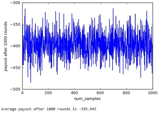
Over 1000 rounds of choosing hit or stick at random, the average payout was found to be around -400 as seen below.
Algorithms and Techniques
Decaying epsilon-greedy Q-learning will be used to solve this problem as the number of states is reasonably small.
- Possible values of sum of agent’s cards [2, 21] = 20
- Face up card of dealer [1, 10] = 10
- Player has usable card [0, 1] = 2
Size of the state space is 400.
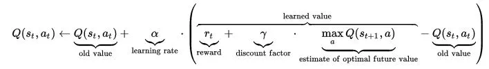
The agent maintains a Q-table which contains an entry for each state and the corresponding Q values for each action possible. When in a particular state of the environment, the agent looks up the maximum Q value for that state and takes the corresponding action. If a state is being reached for the first time, the Q value for each action of that state is initialized to 0 and the action in this case is random as all Q values for the new state are 0. The Q values are then updated based on the reward obtained from the environment using the below formula [4].
Learning rate (alpha)
The agent has to learn based on the reward for a particular action and the learning rate determines how much the agent learns. As can be seen above formula, alpha=0 will make the agent not learn anything while alpha=1 will make the agent consider only the most recent information [4].
Discount factor (gamma)
The discount factor gamma determines the importance of future rewards. A factor of 0 will make the agent “myopic” (or short-sighted) by only considering current rewards, while a factor approaching 1 will make it strive for a long-term high reward [4].
Exploration factor (epsilon)
To ensure the agent learns enough about the environment, it has to explore the environment enough. epsilon determines how much the agent explores by forcing the agent to take a random action with probability epsilon. This ensures the agent reaches new states it hasn’t learned to reach before. However, as the agent learns enough about the environment, it has to minimize exploring and thus a decaying value of epsilon is used. Its value should remain high enough for a while so the agent can sufficiently explore the environment before reducing slowly to a tolerance value. Once epsilon reaches this tolerance value, the exploration stops and the learning is also stopped by making alpha 0.
Number of episodes to train
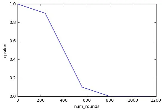
This is a parameter I added to easily tweak the rate of decay of epsilon depending on the number of episodes used to teach the agent. epsilon drops to 90% of its initial value in the first 30% of num_episodes_to_train. epsilon then drops to 10% of its initial value in the next 40% of num_episodes_to_train. epsilon finally becomes 0 in the final 30% of num_episodes_to_train. Here 0 is the tolerance value at which we stop the learning process of the agent by setting alpha to 0. epsilon value decays like in the below graph when the num_episodes_to_train=800.
Benchmark
Assuming the average player uses no strategy and makes a random choice each time (most likely while drunk), the payout at the end of 1000 rounds is simulated in the Open AI environment. This would be the benchmark against which the trained agent in this project will be compared. This exact scenario was simulated above and the benchmark value was found to be -395.9.
III. Methodology
Data Preprocessing
As the Open AI blackjack environment already provides data in a format suitable to be used with the Q-learning algorithm discussed above, no data preprocessing like encoding or modification is necessary. All three features provided are included in the state as all of them are significant and the state space of 400 is small enough as shown above.
Implementation
The algorithm described above in the Algorithms and Techniques section is implemented using Python. The code for this is provided in the accompanying jupyter notebook.
The Agent can be created by passing the environment and the parameters discussed above. The agent is assigned these parameters when created and an empty Q table is created. One of the parameters used is num_episodes_to_train which determines the rate of decay of the parameter epsilon. small_decrement is used to decrease the value of epsilon during the first and last 30% of the episodes to decrease its value slowly. big_decrement is used to reduce the value of epsilon faster during the middle phase of training. The small_decrement value is calculated such that epsilon drops 10% of its initial value over 30% of the episodes and big_decrement is calculated such that epsilon drops between 0.1 x epsilon and 0.9 x epsilon over 40% of the episodes.
The agent has an update_parameters() function which updates epsilon and alpha at the end of each action. small_decrement and big_decrement are used to update the epsilon value based on num_episodes_to_train_left which keeps track of how many more episodes can be used for training. Once, the training is done, alpha is set to 0 to stop the learning process.
There is a choose_action() function that determines which action to take based on the epsilon and the values in the Q-table. This uses the get_maxQ() function which gives the maximum Q value for a particular state. Whenever a new state is seen, it is initialized in the Q table with values for each action set to 0. Using this maximum Q value, the agent returns the corresponding action from the Q table. However, when epsilon is not 0, the agent has to still explore the environment and so the agent takes a random action with probability epsilon. When epsilon is close to 1, this function is more likely to return a random action and when epsilon is close to 0, the action is more likely to be chosen based on the Q-table.
Action from the previous function is fed to the environment which results in a payout passed on to the agent’s learn() function along with the next state in the environment. learn() updates the Q values in the table using these values in the formula Q = Q - Q * alpha + alpha(reward + discount * self.get_maxQ(next_observation)). When alpha is 0, as is the case when there is no more learning to be done, Q values aren’t updated anymore as seen from the formula.
Luckily the original metric chosen for comparing strategies was simple and straightforward enough and didn’t changes after the implementation was complete.
Refinement
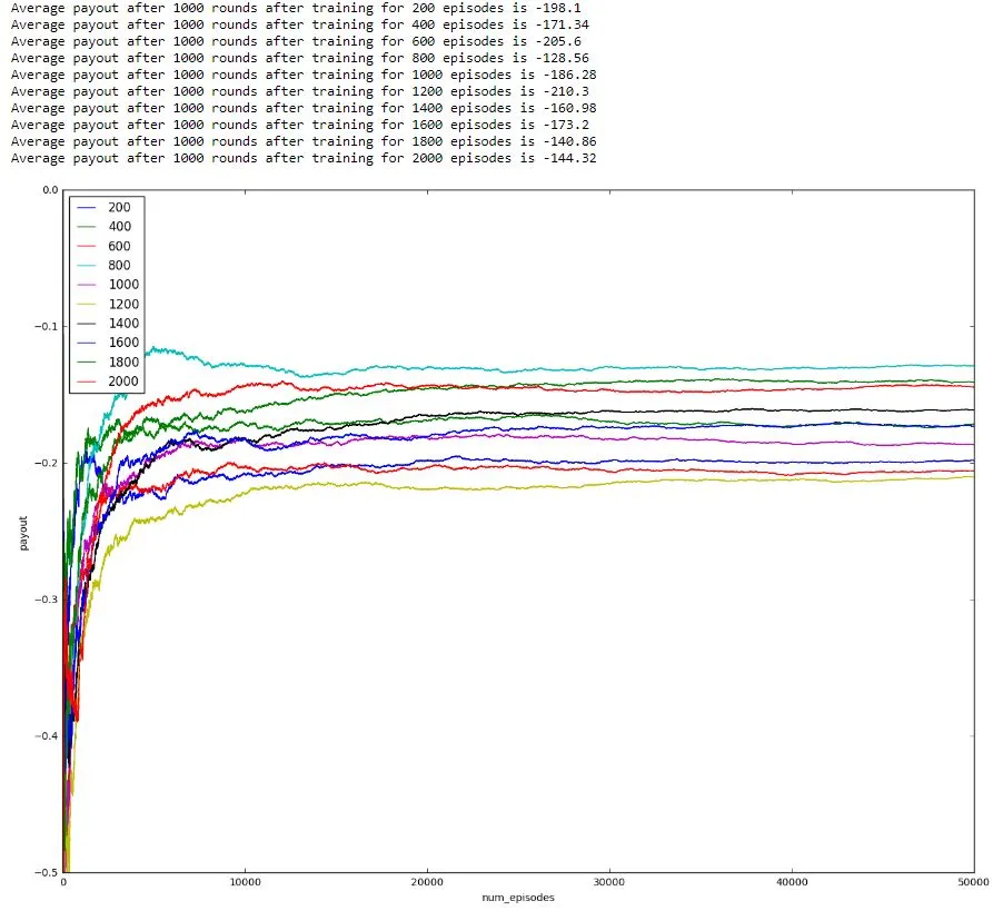
Only one custom parameter (num_episodes_to_train) was tweaked and suitable choices were made for the others. Initial value of epsilon was chosen to be its maximum value of 1. alpha was chosen to a common value of 0.5 and the discount factor gamma was chosen to be 0.2 to keep the agent short-sighted as most of the rounds finish in one, two or three states. The optimum value for num_episodes_to_train was searched over a list of values and chosen to be 800 based on below image. This is because the average payout is highest for this value.
When the value of num_episodes_to_train is too less like 200, it’s payout is low and so is the case when its value is too high. Below image clearly shows that the agent achieves the highest payout when trained over 800 episodes.
IV. Results
Model Evaluation and Validation
The agent is created using the parameters chosen above - the learning rate is set to a common value of 0.5, exploration factor decayed from 1 to 0 over 800 episodes after searching over a range of values and the discount factor is 0.2 to keep the agent short-sighted. The simulations are run 1000 times - each time for 1000 rounds of the game. The agent learns for the first 800 rounds and makes its decisions during the remaining simulations based on its final Q-table.
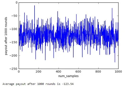
The learned model achieves an average payout per 1000 rounds of around -125 and doing so over a large number of simulations proves the robustness of the model as such a large sample tests the model thoroughly. However, the payout over 1000 rounds of the game is likely to vary a significant amount due to the inherent randomness of the game.
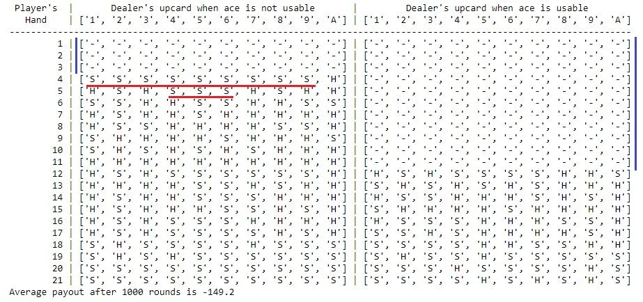
Below is a human readable representation of the strategy learned by the agent. The left half of the image shows the strategy when there is no usable ace (value 1) and the right when there is a usable ace card (ace considered 11). ‘H’ means hit and ‘S’ means stick while ’-’ means the agent hasn’t seen that state while learning. Each row represents the player’s hand and the columns represent the dealer’s ‘up card’. It can be seen that the agent seems to have learned to ‘hit’ when it’s hand is not close to 21. But the agent seems to ‘stick’ a lot more possibly to avoid going bust - a reasonably good strategy. It can also be seen that the strategy is clearly wrong in certain places and some of these are marked by red lines. The agent also did not get a chance to explore some rare states as marked by the blue lines.
Justification
Over 1000 rounds, the average payout was found to be much higher than the benchmark -400 with a value of around -125. This is a significant increase in the payout and proves that the agent has learned to satisfactorily play the game much better than the average casino player.
V. Conclusion
Free-Form Visualization
Below is the average payout achieved by the agent over 1000 trials of playing 1000 rounds of the game. As can be seen, the average payout/1000 rounds mostly lies between -100 and -150 and this fluctuation is an indication of the role luck/chance plays in the game.
Reflection
In this project, a learning agent successfully learned how to play blackjack and collect a payout much better than the average casino player. Blackjack is a card game where the goal is to obtain cards that sum to as near as possible to 21 without going over. They’re playing against a fixed dealer.
Q-learning was used by the agent to continuously update its Q-table during the learning process based on the action taken and the corresponding reward received. The rate at which the agent learns was proportional to the value of its learning rate, alpha which was set to 0.5. The agent first explored the environment rapidly by taking random decisions before relying on its Q-table to make appropriate decisions. This behavior was controlled by the agent’s exploration factor, epsilon. epsilon decreased from it’s initial value of 1 to the tolerance value of 0 in 800 episodes - this was also the number of episodes the agent learned for. The value 800 was found after searching over a list of values between 200 and 2000 and finding the value that produced the maximum payout.
At the end of the above process, the agent achieved a payout of -125 which was significantly bigger than the payout of around -400 received by the average casino player during simulations before the agent was trained.
It was very interesting to see a fairly simple algorithm learn a satisfactory strategy to play blackjack. The code for the agent is general enough to be used as a starting point to solve other environments from Open AI’s gym that have small state spaces.
It was a bit frustrating that the trained agent could not match the performance of the strategies described in [5] despite tweaking the parameters a fair bit.
Improvement
Although the state space is fairly small, using a neural network as a function approximator might result in better payouts at the cost of implementation complexity and processing power/time.
Newer techniques like Double Q-learning or Experience Replay could be tested to see if they improve performance. I recently came across these and should learn more about these to see if they fit this problem.
‘Normal Play Strategy’ from figure 11 here [5] produces a better payout of around -100 per 1000 rounds in this environment so there is certainly room for improvement.
References
[1] Wikipedia entry for Blackjack
[2] The Optimum Strategy in Blackjack
[3] A Markov Chain Analysis Of Blackjack Strategy
[4] Q learning formula
[5] The Evolution of Blackjack Strategies